Power BI Report Server Oct 2020 – “Same key already added” error on refresh

If you’ve upgraded to the October 2020 release of Power BI Server, you might be seeing the following error when you refresh some of your reports:

[0] -1056505856: COM error: mscorlib, An item with the same key has already been added..

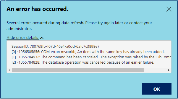
This error appeared when we install the November 18th patch for Power BI Server (15.0.1104.264) and wasn’t present in the original October 2020 release. The especially frustrating part was that reports refreshed just fine in the Power BI Desktop client, and the issue only appeared after publishing the report up to Power BI Server, making it much more difficult to troubleshoot.

However, the resolution ended up being pretty straightforward – there are two different ways to define a connection to a SQL Server database, and if you use both methods in the same data model and then merge the results, Power BI Server has a problem with it (and Power BI Desktop does not). To correct this issue, you need to pick a method and ensure that all the SQL Server connections in your data model use this single method to connect to the database.

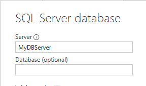
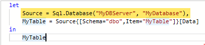
One method is used when you specify a database server, but don’t specify a database:

SQL Server connection with no database specified

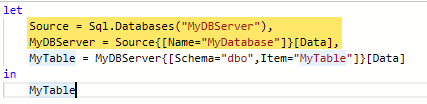
This results in the following M query, with the connection taking up the first two lines (one for server, one for database):

M-query showing two-line database connection

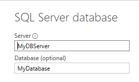
If you specify the database in the connection window instead, it merges the connection statement onto a single line and uses Sql.Database (singular) instead of Sql.Databases (plural). Since you’re required to specify a database name when you provide a SQL query, so a custom query always uses this one-line method to connect:

Connection window showing database name
M-query database connection merged into a single line

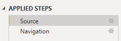
Regardless of whether you enter the database name (and have the one-line connection method) or don’t enter a database (and use the two-line method), it looks exactly the same in the step window in Power Query:

“Source” is the database connection, whether it’s one or two lines. Navigation is the step that specifies the table/view you’re connecting to, and is the “MyTable” step in the examples above.

I’d recommend using method two for all your connections, as that’s what’s needed to run a specific SQL query – if any of your data sources and query-based and not just selecting a table, you’ll have to use this approach.

I hope this helps somebody else! While I’d love it if Power BI Server avoided errors like this one, I’d also really appreciate it if Power BI Server and Desktop used the same code for shared functionality so that you can be aware of issues before you publish your reports and they fail to refresh.

This took some frustration to resolve and I’m thankful for finally finding the resolution to this issue through a bug report that “JeanMartinL” had filed: https://community.powerbi.com/t5/Issues/BUG-Report-Server-refresh-fails-if-data-source-are-created/idi-p/1528954. Whoever you are, thank you!


Removing columns named “Column” when importing Excel files with Power Query

When importing Excel files using Power Query, any columns without a name in the first row will end up titled “Column123”, with an number at the end that increments for each column. This happens whether they contain actual data, or whether they’re just formatted columns that contain nothing at all.

Example of imported Excel file with two named columns and two just called “Column”.

If you’re importing a single file, you can rename or delete these columns as you need to. However, if you’re importing an entire folder of Excel files or the format changes unpredictably, you may want to automatically remove all o these columns at the end.

To do this, you’ll use the “Advanced Editor” to add a line of M-code:

"Remove Columns Named Column" = Table.RemoveColumns(#"Promoted Headers", List.FindText(Table.ColumnNames(#"Promoted Headers"), "Column")), 
After adding the new step, columns named “Column” are now gone.

After you add this step, you may need to modify your “Changed Type” step to only set the type on columns you’re keeping, as it automatically mentions every single column by name.

Adding this step will remove the additional columns, dynamically, every time the data is imported. Now when you import a folder full of Excel files and some of them contain additional columns or rogue formatting, the step will drop them if they don’t get named.

Import first sheet of an Excel workbook into Power Query, regardless of its name

I recently had to import a large number of Excel workbooks into Power Query (using “From Folder” – if you haven’t used this feature, it’s a huge time-saver when you’ve got a ton of matching files to import). The problem was that each workbook had a different name for the first tab and the import process gets data from tabs with the same name (assuming all your files match).

By default when you create a workbook, Excel names the first sheet “Sheet1”, but if the files you’re importing have sheets with different names, you can tell Power Query to load the first sheet of each file, regardless of the name – here’s the process (skip to step 5 to see the specific M-query solution):

  1. Select “Get Data” -> “From File” -> “From Folder” – this lets you import all the files from a folder at once (assuming their format matches).
  2. Select the folder where your files are stored (I have three files in the folder in this example).
  3. Select an example file and which sheet you’d like to import – this is what you’ll use to create your transformations (before the files are merged together) – in this example, my sheet is called “Bob’s sheet” (which is specific to just that single file).
  4. When you select “Import”, you’ll receive the error “[Expression.Error] The key didn’t match any rows in the table.” – this is because the other workbooks don’t contain any sheets with that name (though the error is a bit cryptic).
    If you double-click on the “Data Files” query with the error, you can see that it loaded the data from the first file, but nothing from the others:
  5. To correct this issue and tell Power Query to just use the first tab in the workbook in every case, open the “Transform Sample File from Data Files” query and click “Advanced Editor”.
  6. You’re now looking at the M-query behind this object (if you want it, here’s a great video on M if you’ve never worked it before and want a primer – I watched a bunch of different videos and this one really connected the dots for me). The section with the sheet name is highlighted:
    Replace the highlighted text with “Item=Source{0}[Item]” so that it looks like this:
    (The “0” refers to the first sheet – if you want the second sheet, you’d use “1” and so on). If you’re using an XLS file rather than an XLSX file, the text looks a little bit different: “Name=Source{0}[Name]“. The XLSX file has a Name field as well, but it can vary from the “Item” column.
  7. Once you make change, you can see in the Power Query window that it’s now getting data from every file.
  8. Once you click “Close and Load” to get back to Excel, click on the “Refresh All” button to force a data refresh and you’ll see it import all the files, regardless of their sheet name:

That’s it – you’re pulling in all the workbooks regardless of their sheet name!

I’d never used the “From Folder” feature, but I’d definitely recommend trying it out – it was a huge time-saver for me and allowed me to import hundreds of matching Excel files into a single model in minutes!

Update: When you’re using older XLS files

Somebody brought to my attention that this technique doesn’t work when you’re using XLS files, only when you’re using the XLSX/XLSB format (I won’t call it new as it’s been around since Office 2007, but still – newish).

If you’re using XLS files, you need to change step 6 slightly as M uses a different syntax to drill into sheets in those files. Here’s what the M query looks like when you drill in manually:

Replace the highlighted portion ([Name=”Sheet1″]) with just an index number – “0” in this case:

Once you do that, Power Query will drill into the sheet in the the first row of your dataset.

However, I did notice an issue – the sheet in position “0” wasn’t the first sheet in the workbook. I added a number of sheets in my Excel doc, but I did it them in a random order (I renamed “Sheet1” to “Original” and then created the others in the order they’re named):

However, when you import the workbook in Power Query, the physical order isn’t reflected – it seems to be the order they were created, but with the original sheet always last (not sure what the thinking is there – maybe something in the physical file format?):

If you want the “Original” sheet, you can use the Power Query step “Keep Bottom Rows” and give it a value of “1”:

If you want one of the other sheets, though, and the name keeps changing, I’m not sure how you’d handle ensuring you get the right one. If you’ve got suggestions, I’d love to hear them and I’ll include them here!

Update 2

Another question from the comments – what if you want to get the last sheet in the workbook, not the first one? We can make that happen with one additional line right after Source and right before the line where you select the sheet:

"Kept Last Rows" = Table.LastN(Source, 1),

This is the command you get when you select “Keep Rows” -> “Keep Bottom Rows” from the toolbar up top, and you’ll be left with a single row to drill into. You’ll still need to drill into it as Row 0 so that it will work no matter what the sheet name is.

Migrate database indexes to a new file group

I recently had to mass-migrate all the indexes from a database to a new file group since we’d added some additional storage to our database server. I found this article at SQL Server Central (unfortunately, registration required, so I’ve included a copy of the original script in the download at the end). While it worked okay, there were some things I didn’t like about it:

  • Assumed 90% index fill rate
  • “Moved” indexes were all created as non-unique, regardless of original
  • Fail during index creation left you without an index (drop and then create, with no rollback)
  • Table was un-indexed during the move (index dropped and then created)
  • Script re-created indexes without any “Included” columns, even if original index had them

To address these limitations, I rebuilt the process using that script as a starting point. The new script:

  • Uses 90% fill rate by default, but if the original index had a different rate specified, it will use that
  • Re-creates indexes as unique if the source index was unique
  • Rollback problem resolved – new index is created with different name, old index is dropped, and then new index is renamed, all in a TRY-CATCH block
  • Since the new index is created and then the old one dropped, table indexing remains “online” during the move
  • Migrates “Included” columns in index
  • Updated the script to use SYS views (breaks compatibility with SQL 2000, since SYS is 2005/2008/beyond only)
I welcome any feedback on the script, and would love to know if you see any improvements that should be made.

Download .SQL scripts (contains both Original and Modified scripts)